 So what is a hexacontatetrapole moment, anyway?
A sum of sines and cosines can be used to model period functions, given the correct coefficients (a Fourier series). Similarly, a special set of polynomials known as Legendres can model functions in a spherical coordinate system: specifically, spherical harmonics. In our lab, we care about spherical harmonics when we're talking about atomic orbitals--these charge clouds can be modeled using a series of Legendres. The collection of necessary parameters are known as the multipole moments.
Multipoles have many uses throughout the physical sciences. One common example comes from computational chemistry: predicting the electric potential (voltage) field due to a complex molecule. You could find the components of the field at each point due to every atom, but this becomes a tremendous task with a large molecule. Instead, the molecule can be decomposed into a handful of multipole moments which provide simple equations for predicting the field.
In essence, multipoles describe how much something behaves like another system that we can predict easily.
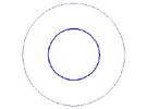 We start by asking, "How much does this act like a ball of charge?" In that case, the potential field is distributed evenly in all directions, and our multipole moment is an estimate of the total charge.
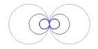 Next, we ask about how much the field behaves like a dipole: two opposite charges seperated by a small distance. In this case, the field has two bulbous ends, one with a positive potential and the other with negative potential. This multipole moment is something like the center of charge, giving us a clue to the distance between our origin and the center of charge. In some sense, the dipole is similar to the center of mass for a solid object.
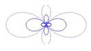
 As more charges are arranged together, they start creating strange looking fields. The beauty of the mathematics is that all the fields fit together to create a more complete picture of the field. We have information about the charge and center of mass from the first two poles, then keep adding finer and finer details until we have an adequate idea of the field's behavior. In the case of our hexacontatetrapole, that's seven poles deep, and we have an excellent measurement of how the system is behaving.
In an experiment, we start with data, extract multipoles, and try to reassemble the original field. Depending on the mathematics, this can give a single field solution or a set of solutions. While we can go backwards in some cases, the important information is not necessarily the original field, but how that field behaves. This is again where the multipoles come in handy: based on the multipole data, we can anticipate a reaction to the field without knowing what it true shape is, and we can gather hints about what the shape might be.
Let's take three examples, and look at what we can predict about the fields based on the multipoles. We'll use a football, a discus, and a bowling pin as familiar examples with differing poles. Each has a well defined axis of rotation, but differ in their symmetries around an equatorial axis. The football is longer in the axial direction, whereas the discus is wider in the equatorial direction than it is long. The bowling pin is not symmetric about its equator, since one end bulges out much more than the other.
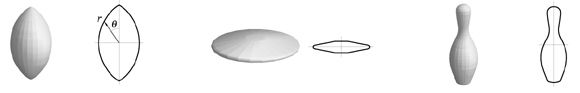
To calculate the multipoles, we took a photograph of each object, then plotted points along its outline to simulate data. Next, we used integration to fit multipoles to the data sets, similar to the experiments in our lab. Those values are listed in the following table:
| Order | Name | Football | Discus | Bowling Pin |
|---|---|---|---|---|
| 0 | Monopole | 1 | 1 | 1 |
| 1 | Dipole | 0 | 0 | -3.15 x 10⁻² |
| 2 | Quadrupole | 2.35 x 10⁻³ | -4.13 x 10⁻³ | 5.22 x 10⁻³ |
| 3 | Octupole | 0 | 0 | -1.56 x 10⁻⁴ |
| ... | ||||
| 6 | Hexacontatetrapole | 1.38 x 10⁻⁷ | -4.84 x 10⁻⁷ | 6.61 x 10⁻⁷ |
The first thing to notice is that if the object or field is symmetric, like the football and discus, all the odd-ordered multipoles are zero. These odd multipoles are all based on Legendre polynomials that are non-symmetric, so we wouldn't expect them in a symmetric object. Secondly, the sign of the multipole indicates whether there is an addition or subtraction from the field. The football has positive multipoles, and continues to grow slowly in the axial direction. The discus alternates sign, causing it to shrink a small amount more than it grows in the axial direction, making it wider in the equatorial direction.
Great, we can calculate interactions. But what about the original field?
Multipoles can give us a good idea of how the field behaves without having to know the original field. In some cases, we can actually go backwards to create a field. For our sports balls, we can only generate one field of an infinite number of fields, but we'll see that given some guesses about the original size, our generalizations about what multipoles come from which shape will hold.
Again using multipoles, we can create spheres of varying density that yield pure multipole moments. A sphere with a density that varies in the same way as a dipole will end up with only a dipole moment, nothing else. By assembling these spheres together with the right weights, we create a new sphere that is composed of only pure multipole moments, and will thus yield the same multipoles.
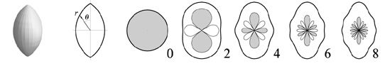
Above is a reconstruction of the football, assuming a radius of 15 cm. The index is the highest order of multipoles used in that reconstruction, with zero being the monopole and six being the hexacontatetrapole. We've taken the mutipole spheres and graphed radius as a function of density; these are the thick black lines. Each additional multipole is shown in grey and white, where grey is an addition and white is a subtraction. These illustrate how the multipoles influence the overall shape. With the football, the "shape", or the thick black line, becomes longer in the axial direction, and has the general shape of a football.
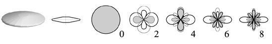
The discus is quite a bit different from the football. It gets shorter in the axial direction and slowly grows in the equatorial direction. The shape line is complex, so it's hard to say that at this order we've got a discus, but many of the characteristics are the same. Note that this shape gives the same multipoles as the discus we are familiar with. In this reconstruction, the bulbous ends of the multipoles along the axis alternate positive and negative, just as the multipole moments did. However, there is always a grey positive addition along the equatorial plane.
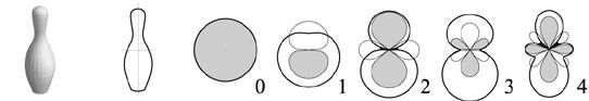
The bowling pin is unique in that it has both odd and even multipoles. As the reconstruction progresses, the bottom end becomes larger and the top end becomes slightly smaller. The neck region shrinks, and the net shape resembles the beginnings of a bowling pin. The multipoles have signs such that the grey positive addition is towards the bulbous end.
These examples illustrate that you can get a general sense of the original field based on the multipoles, but (depending on the mathematics) the original field may not be reconstructable.
So, what is a hexacontatetrapole?
Despite the long name, it's just the 7th layer (6th order) of detail for a system represented by multipoles. It gives another level of information for understanding exactly what's going on in an interaction. In the end, we even have a better idea of what the charge cloud looks like in the system under study.
For our lab, and many other areas of physical science, multipoles are useful tools.